Pruning and Sparsity¶

Abstract

Introduction to Pruning
- What is pruning?
- How should we formulate pruning?
Determine the Pruning Granularity
- In what pattern should we prune the neural network?
Determine the Pruning Criterion
- What synapses/neurons should we prune?
Determine the Pruning Ratio
- What should target sparsity be for each layer?
Fine-tune/Train Pruned Neural Network
- How should we improve performance of pruned models?
System Support for Sparsity
- EIE: Weight Sparsity + Activation Sparsity for GEMM
- NVIDIA Tensor Core: M:N Weight Sparsity Sparsity
- TorchSparse & PointAcc: Activation Sparsity for Sparse Convolution

MLPerf (the Olympic Game for AI Computing)

benchmark, 基于 BERT, 要求保持 99% 的 accuracy，衡量加速比。可以发现 open division 相较于 closed 获得了 4.5x 的加速比。

closed division: 只靠硬件加速，不能改变网络结构（比如权重数量、精度）。
open division: 可以改变网络结构，比如剪枝、降低精度、压缩等技巧。

可以看出，通过剪枝改变网络结构可以显著地提网络性能。

Introduction to Pruning¶

Motivation: 内存很昂贵，会消耗大量的能源。
Idea: Make neural network smaller by removing synapses and neurons.

我们去掉神经网络里的一些小的连接（去掉即让权重为 0），使网络变得更小。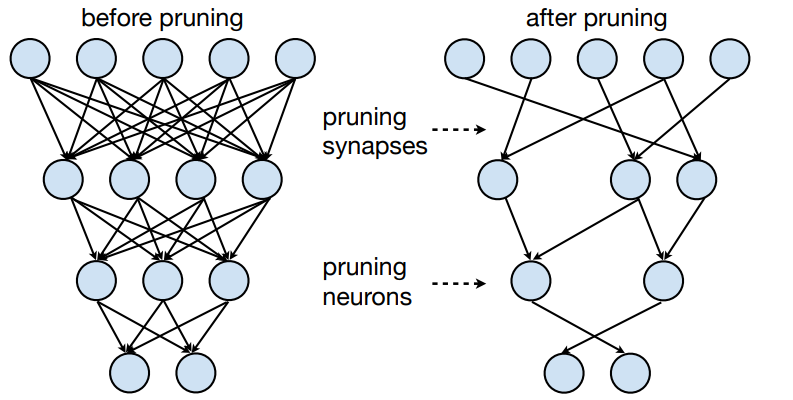
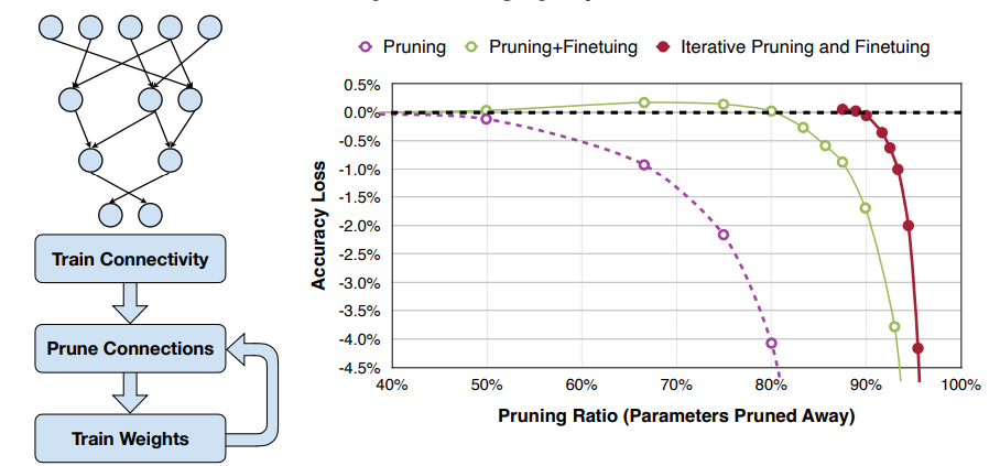
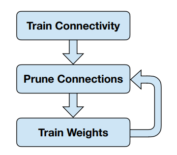
大体流程如下：
- Train Connectivity 首先我们训练至收敛
- Prune Connections 然后我们去掉一些连接
- Train Weights 最后我们重新训练权重
- 第 3 步执行完后可以继续第 2 步，如此迭代。
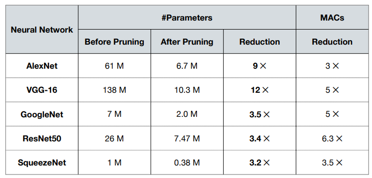
Example

可以看到不同的网络有不同的 pruning ration，其中 VCG-12 可以达到 12x 的 reduction，说明较大的网络内部的冗余也更多。对于较小的网络如 SqueezeNet，我们依然可以达到 3.2x 的 reduction。

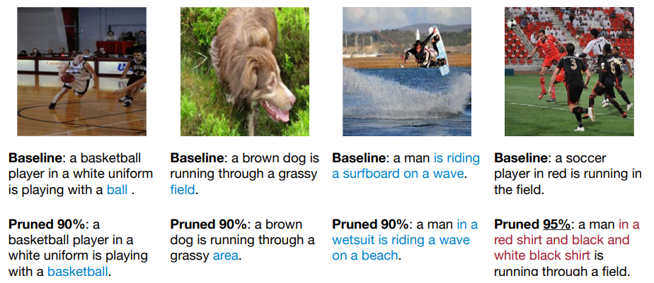
Pruning the NeuralTalk LSTM does not hurt image caption quality.

即使我们减去了大部分连接，但是如果这个比例在接受范围内，那么不会影响分类的质量。如下面的前三个图，我们可以看到剪枝后提取的信息足够用来识别物体。但是对于第四个图，我们剪枝了 95%，导致了信息捕获不足。
通常我们将剪枝表示为

\[ \arg\min\limits_{\mathbf{W}_p}L(\mathbf{x};\mathbf{W_p})\quad s.t.\ \|\mathbf{W}_p\|_0\leq N \]

其中，
- \(L\) 是神经网络训练的目标函数。
- \(\mathbf{x}\) 是输入，\(\mathbf{W}\) 是原始权重，\(\mathbf{W}_p\) 是剪枝后的权重。
- \(\|\cdot\|_0\) 表示非零元素的个数，\(N\) 表示我们希望有多少权重保持非零。

Determing the Pruning Granularity¶

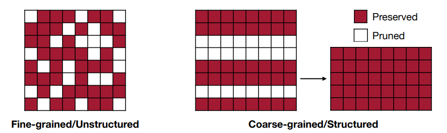
不同粒度的剪枝会有不同的效果，如下图所示：
- Fine-grained/Unstructured:
  - More flexible pruning index choice
  - Hard to accelerate (irregular)
- Coarse-grained/Structured:
  - Less flexible pruning index choice (a subset of the fine-grained case)
  - Easy to accelerate (just a smaller matrix!)
上面是对于 2D 的矩阵，对于卷积层，我们有 4 个维度 \([c_0, c_i, k_h,k_w]\)，这给了我们更多的剪枝粒度的选择。
- \(c_i\): 输入通道数; \(c_0\): 输出通道数; \(k_h,k_w\): kernel 的高和宽。
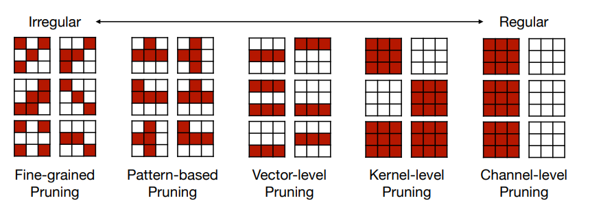
- Fine-grained Pruning
  - 逐个元素选择是否剪枝，通常可以得到更高的剪枝率。但是需要注意的是，参数的减少不能直接转为 speed up，还需要考虑硬件上的效率。
  - 细粒度的剪枝只能在某些特定硬件上得到加速（如 EIE），但是在 GPU 上不能得到加速。
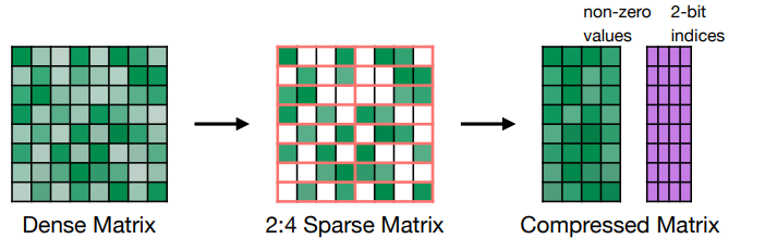
- Pattern-based Pruning: N:M sparsity
  - N:M sparsity 是指每连续 M 个元素，我们修建掉 N 个。常用的情况是 2:4 sparsity(50%).
  - 这种剪枝方式可以在 NVIDIA’s Ampere GPU 架构上得到加速。如下图所示，我们会存修剪后的非零值，同时有一个额外的索引块来存非零值的原始位置。
  - 通常可以保持精度（在各种任务中经过测试）。
- Channel Pruning
  - 直接去掉某些通道，好处是可以直接获得加速（相当于降低了 \(c\) 的大小）。
  - 但是剪枝率也较低。这个方法被广泛使用，因为足够简单。
  - 对于不同层，我们可以采用不同的剪枝率，这样能在相同的精度下获得更低的延时。

Determine the Pruning Criterion¶

Selection of Synapses to Prune¶

当剪枝参数时，我们希望移除不太重要（less important）的参数，这样我们剪枝后的神经网络能获得更好的性能。
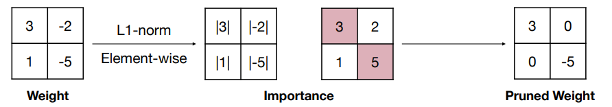
Magnitude-based Pruning
- 启发式的剪枝准测，我们把认为有更大绝对值的权重更重要。
- 对于 element-wise 的剪枝，\(Importance=|W|\).
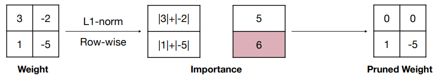
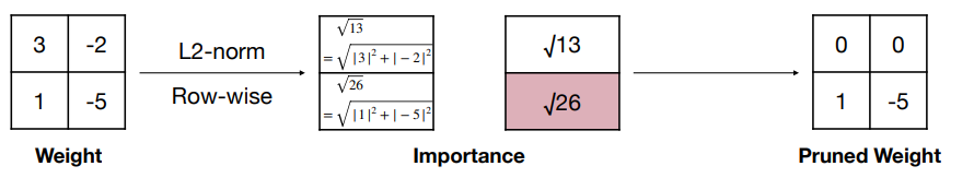
- 对于 row-wise 的剪枝，\(Importance=\sum\limits_{i\in S}\sum|w_i|\) 或者 \(Importance=\sum\limits_{i\in S}\sqrt{\sum|w_i|^2}\). 其中 \(\mathbf{W}^{(S)}\) 是权重 \(\mathbf{W}\) 的 \(S\) 结构集合，这里分别是 L1 和 L2 范数。
- 也可以使用 Lp 范数，即 \(\|\mathbf{W}_p^{(S)}\| = \left(\sum\limits_{i\in S}|w_i|^p\right)^{1/p}\).
Example
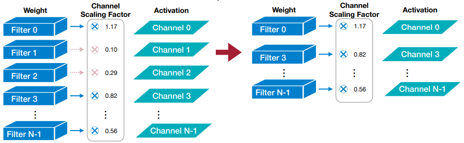
Scaling-based Pruning
- 这个剪枝方法用于 filter pruning。在卷积层里每个 filter 都有一个 scaling factor 缩放因子（可训练的），把这个因子和输出通道的输出乘起来。缩放因子较小的通道将被修剪掉。
- 这个缩放因子可以用在 BatchNorm 层里。
Example
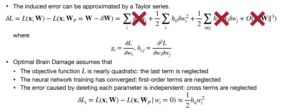
Second-Order-based Pruning
- 通过泰勒级数推导误差，随后通过 Hessian 矩阵的特征值来评估权重的重要性。

Selection of Neurons to Prune¶

我们还可以修剪神经元/激活值（粗粒度，因为去掉神经元相当于把所有相关的连接权重去掉了），类似地我们希望移除不那么有用（less useful）的神经元。
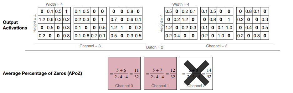
Percentage-of-Zero-Based Pruning
- ReLU 激活函数会在输出里产生 0，因此我们可以采用 Average Percentage of Zero activations (APoZ) 来衡量权重的重要性。APoZ 越小，说明权重越重要。
Example

在这里我们基于 channel 做修剪：可以看到 channel 2 的 APoZ 最小，因此我们可以修剪掉这个 channel。
Regression-based Pruning
- 因为大模型下微调不那么容易，我们可以单独关注某层，通过回归的方法，最小化重建（即从输入到输出）对应层输出的 reconstruction error 误差。
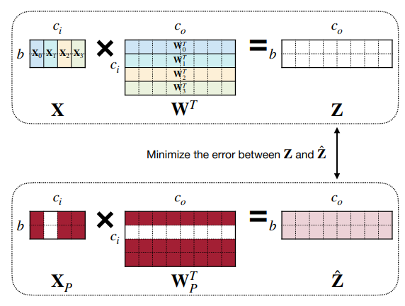
- 令 \(\mathbf{Z}=\mathbf{X}\mathbf{W}^\top=\sum\limits_{c=0}^{c_i -1}\mathbf{X}_c \mathbf{W}_c^\top\), 那么我们要做的就是
  
  \[ \arg\min\limits_{\mathbf{W}, \beta}\|\mathbf{Z}-\hat{\mathbf{Z}}|_F^2 = \|\mathbf{Z} - \sum\limits_{c=0}^{c_i-1}\beta_c \mathbf{X}_c \mathbf{W}_c^\top\|_F^2 \quad s.t.\ \|\beta_0\| \leq N_c \]
  - \(\beta\) 是长为 \(c_i\) 的向量的通道系数，\(\beta_c=0\) 说明我们修剪掉了通道 \(c\)。
  - \(N_c\) 是我们希望保留的通道数。
  - 解决这个问题，可以通过：
    - 固定 \(\mathbf{W}\), 解出 \(\beta\) 用于通道选择。
    - 固定 \(\beta\)，解出 \(\mathbf{W}\) 用来最小化重建误差。

Determine the Pruning Ratio¶

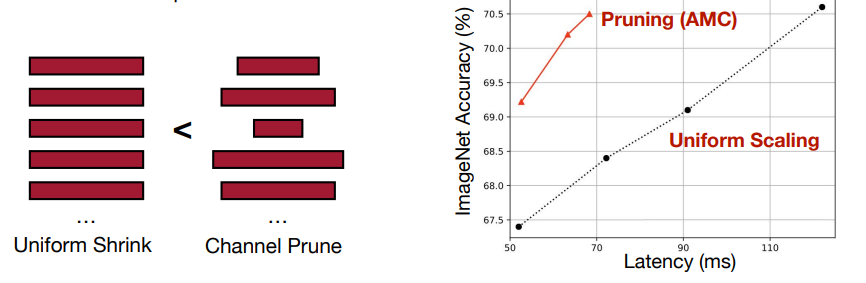
Non-uniform pruning is better than uniform shrinking. 非规则的剪枝比规则的剪枝更好。
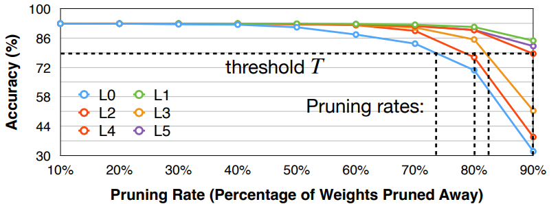
需要分析每一层的 sensitivity 敏感度，然后根据 sensitivity 来决定各层的剪枝率。有的层更加敏感（比如第一层），有的层冗余更多（比如全连接层）。
- 选择模型中的 \(L_i\) 层，剪枝 \(L_i\) 层至剪枝率 \(r\in \{0, 0.1, 0.2, \ldots, 0.9\}\)（或者使用其他步长），随后观察模型的精确度下降情况 \(\nabla Acc_r^i\)。重复这个步骤知道所有层都被分析结束。
- 最后我们可以选择一个 threshold \(T\), 即精度至少要保持在 \(T\) 以上，然后为每一层选择对应的剪枝率。
- 这是一种启发式的方法。同时这里我们假设了不同的层之间是相互独立的，不会互相干扰。但实际上层与层之间存在相互关系，因此这样的方法并不是最优的。
Example

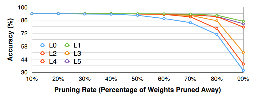
Note

需要注意的是剪枝率并没有反映 layer size，比如上面的例子中虽然 L1 可以很激进地修剪，但可能 L1 本来就只有 20 个参数，这样的剪枝率并不会对整个网络的大小产生很大的影响。

在 LLM(Transformer) 背景下，各个层都是 homegeneous 的，即每层的大小不会有太大的变化。但是对于 CNN，每层的大小都是不同的，因此我们需要考虑每层的 size。
Automatic Pruning
- 在过去，剪枝的比例是人工选择的，需要我们通过实验试错来确定最终比例。我们希望有一个 push-the-button 的方法来自动选择最佳的剪枝比例。
- AMC (AutoML for Model Compression) 是一个自动选择剪枝比例的方法，它通过强化学习来选择最佳的剪枝比例。
  
  这里实际上我们会把 reward 设为 \(-Error*\log(FLOP)\) 用来平衡精度和 FLOP（近似延时）的关系。
  
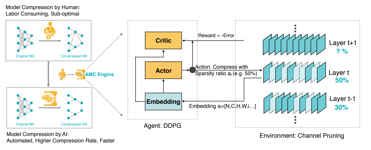
  最终我们可以得到比人工修剪更好的结果。
- NetAdapt: A rule-based iterative/progressive method

Fine-tune/Train Pruned Neural Network¶

剪枝后模型的精度会下降，我们需要微调剪枝后的模型来恢复精度，并可以尝试让剪枝率更高。
Learning rate for fine-tuning is usually 1/100 or 1/10 of the original learning rate.

经验上会这么设置微调时的学习率，因为在剪枝前模型已经收敛了，我们不需要太大的学习率来调整模型。
Iterative Pruning

先训练到收敛，随后进行剪枝。剪枝后再次训练至收敛。随后可以进一步提高剪枝率，如此迭代。
Regularization
- 训练或者微调时，我们会把正则化项 regularization 加到损失上。
  - 惩罚非零参数，目的是尽可能地多修剪参数。
  - 鼓励更小的权重，这样下一轮迭代就可能修剪掉这些权重。
- 常见的正则化 \(L'=L(\mathbf{x};\mathbf{W})+\lambda |\mathbf{W}|\), \(L'=L(\mathbf{x};\mathbf{W})+\lambda \|\mathbf{W}\|^2\)

System Support for Sparsity¶

EIE: Weight Sparsity + Activation Sparsity for GEMM¶

The First DNN Accelerator for Sparse, Compressed Model

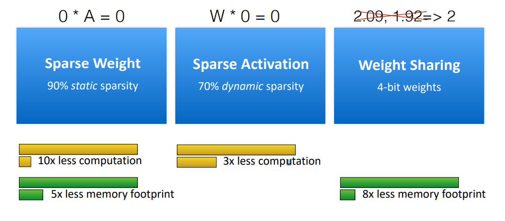
0 是一个特殊的值，因为 0 的权重/激活值不需要计算/存储（结果肯定为 0），从而可以节省计算和存储。

why weight 10x less computation while 5x less memory footprint

因为为了表示 sparse matrix，我们还需要存索引，因此存储空间的节省不如计算量的节省。
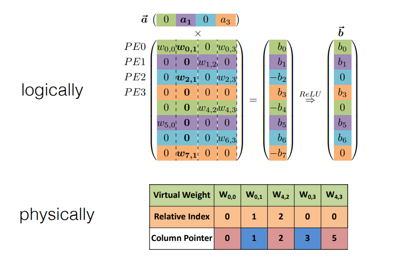
Parallelization on Sparsity

Example

这里 relative index 表示和上一个非零值的相对位置，column pointer 表示是否开始新的一列。
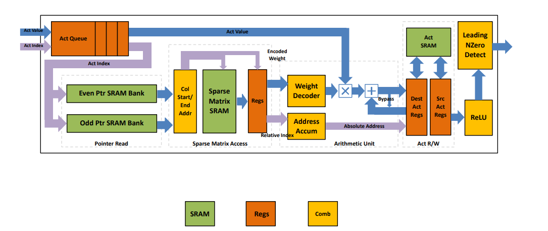
Micro Architecture for each PE

总结 EIE

Pros:
- EIE demonstrated that special-purpose hardware can make it cost-effective to do sparse operations with matrices that are up to 50% dense
- EIE exploits both weight sparsity and activation sparsity, not only saves energy by skipping zero weights, but also saves the cycle by not computing it.
- EIE supports fine-grained sparsity, and allows pruning to achieve a higher pruning ratio.
- Aggressive weight quantization (4bit) to save memory footprint. To maintain accuracy, EIE decodes the weight to 16bit and uses 16bit arithmetic. W4A16 approach is reborn in LLM: GPTQ, AWQ, llama.cpp, MLC LLM
Cons:
- EIE isn’t as easily applied to arrays of vector processors — improve: structured sparsity (N:M sparsity)
- EIE’s Control flow overhead, storage overhead — improve: coarse grain sparsity
- EIE only support FC layers - actually reborn in LLM
- EIE fits everything on SRAM - practical for TinyML, not LLM

The first principle of efficient AI computing is to be lazy!

Avoid redundant computation, quickly reject the work, or delay the work.

我们设想未来的人工智能模型将在各种粒度和结构上稀疏。与专门的加速器共同设计，稀疏模型将变得更加高效和易于访问。

Related Work

Generative AI: spatial sparsity [SIGE, NeurIPS’22]
Transformer: token sparsity, progressive quantization [SpAtten, HPCA’21]
Video: temporal sparsity [TSM, ICCV’19]
Point cloud: spatial sparsity [TorchSparse, MLSys’22 & PointAcc, Micro’22]

NVIDIA Tensor Core: M:N Weight Sparsity Sparsity¶

TODO

TorchSparse & PointAcc: Activation Sparsity for Sparse Convolution¶