Query Processing

Abstract

• Basic Steps in Query Processing
• Measures of Query Cost
• Selection Operation
• Sorting
• Join Operation
• Other Operations
• Evaluation of Expressions

Basic Steps in Query Processing

经过语法分析、语义检查翻译成关系表达式，经过查询优化转化成执行计划（目标代码），由求值引擎得到输出。

Example

逻辑优化：把选择运算往叶子上推；先连接的是结果比较小的。
An evaluation plan defines exactly what algorithm is used for each operation, and how the execution of the operations is coordinated.

经过代价估算，决定使用哪个算法的代价最小。如上图左边使用了 B+ 树索引，右边使用了线性扫描。
pipeline 表示最下面两步可以流水线，即并行计算。
（火山模型）

Measures of Query Cost

Typically disk access is the predominant cost, and is also relatively easy to estimate.
忽略 CPU cost.
Measured by taking into account

• Number of seeks
• Number of blocks read
• Number of blocks written
  通常写的时间比读的时间久，因为我们可能需要检验写的结果

For simplicity we just use the number of block transfers from disk and the number of seeks as the cost measures

• \(t_T\) – time to transfer one block
• \(t_S\) – time for one seek
• Cost for b block transfers plus S seeks \(b * t_T + S * t_S\)

We often use worst case estimates, assuming only the minimum amount of memory needed for the operation is available.
即假设缓冲区最小的时候，而且都是从文件中读取而非从 buffer 中读取。

Selection Operation

File scan

Algorithm A1 (linear search). Scan each file block and test all records to see whether they satisfy the selection condition.
（假定数据块都是连续存放的）

• worst cost = \(b_r*t_T+t_S\)
  \(b_r\) 是要找的块的数量
• average cost = \(b_r/2*t_T+t_S\)
  这里如果搜索的是 key, 那我们扫到这个记录就可以停止。

Index scan

A2 (primary B+-tree index / clustering B+-tree index, equality on key).
在主键上查找

cost = \((h_i+1)* (t_T+t_S)\)

主索引, key 上的等值查找

这里的高度从 1 开始（+1 表示最后到叶子节点，需要从磁盘中读）

A3 (primary B+-tree index/ clustering B+-tree index, equality on nonkey).
Records will be on consecutive blocks
此时索引的值不是主键. b 表示搜索码对应的记录数量。

cost = \(h_i *(t_T+t_S) + t_S + t_T *b\)

主索引, nonkey 上的等值查找

A4 (secondary B+-tree index , equality on key).

cost = \((h_i + 1) * (t_T + t_S)\)

辅助索引, key 上的等值查找

A4’ (secondary B+-index on nonkey, equality).

Cost = $(h_i + m+ n) * (t_T + t_S) $
这里 m 表示放指针的块的数量, n 表示对应磁盘里的记录的数量。

辅助索引, nonkey 上的等值查找

Selections Involving Comparisons

查询 \(\sigma_{A\leq V}(r)\) (or \(\sigma_{A\geq V}(r)\))

A5 (primary B+-index / clustering B+-index index, comparison). (Relation is sorted on A)

• 首先找到第一个 \(\geq v\). 的值
• 把后面的块顺序读进去 Cost = \(h_i * (t_T + t_S) + t_S + t_T * b\) (同情况 3)

主索引, key 上的比较

A6 (secondary B+-tree index, comparison).
情况类似 A4

辅助索引, nonkey 上的比较

Implementation of Complex Selections

Conjunction \(\sigma_{\theta_1} \wedge \ldots \wedge_{\theta_n}(r)\)
可以线性扫描，或者利用某个属性的 index 先查询，把符合的读到内存中，再检查其他属性。
如果有很多个属性都有索引，我们选择中间结果少的。

A7 (conjunctive selection using one index).

• Select a combination of \(\theta_i\) and algorithms A1 through A6 that results in the least cost for \(\sigma_{\theta_i}(r)\).
• Test other conditions on tuple after fetching it into memory buffer.

A8 (conjunctive selection using composite index).
Use appropriate composite (multiple-key) index if available.
利用复合索引

A9 (conjunctive selection by intersection of identifiers).
对每个索引都进行查询，将结果拼起来

Algorithms for Complex Selections

• Disjunction: \(\sigma_{\theta_1} \vee \ldots \vee_{\theta_n}(r)\)
  A10 (disjunctive selection by union of identifiers).
  • Applicable if all conditions have available indices.
  • Otherwise use linear scan.
  • Use corresponding index for each condition, and take union of all the obtained sets of record pointers.
  • Then fetch records from file
• Negation: \(\sigma_{\neg \theta}(r)\)
  • Use linear scan on file
  • If very few records satisfy \(\neg \theta\), and an index is applicable to \(\theta\) Find satisfying records using index and fetch from file

Bitmap Index Scan

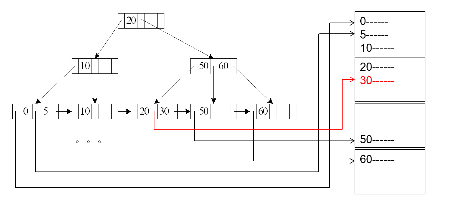
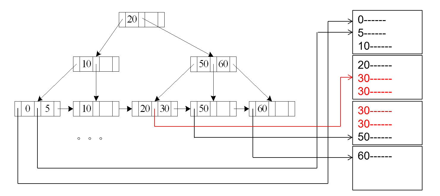
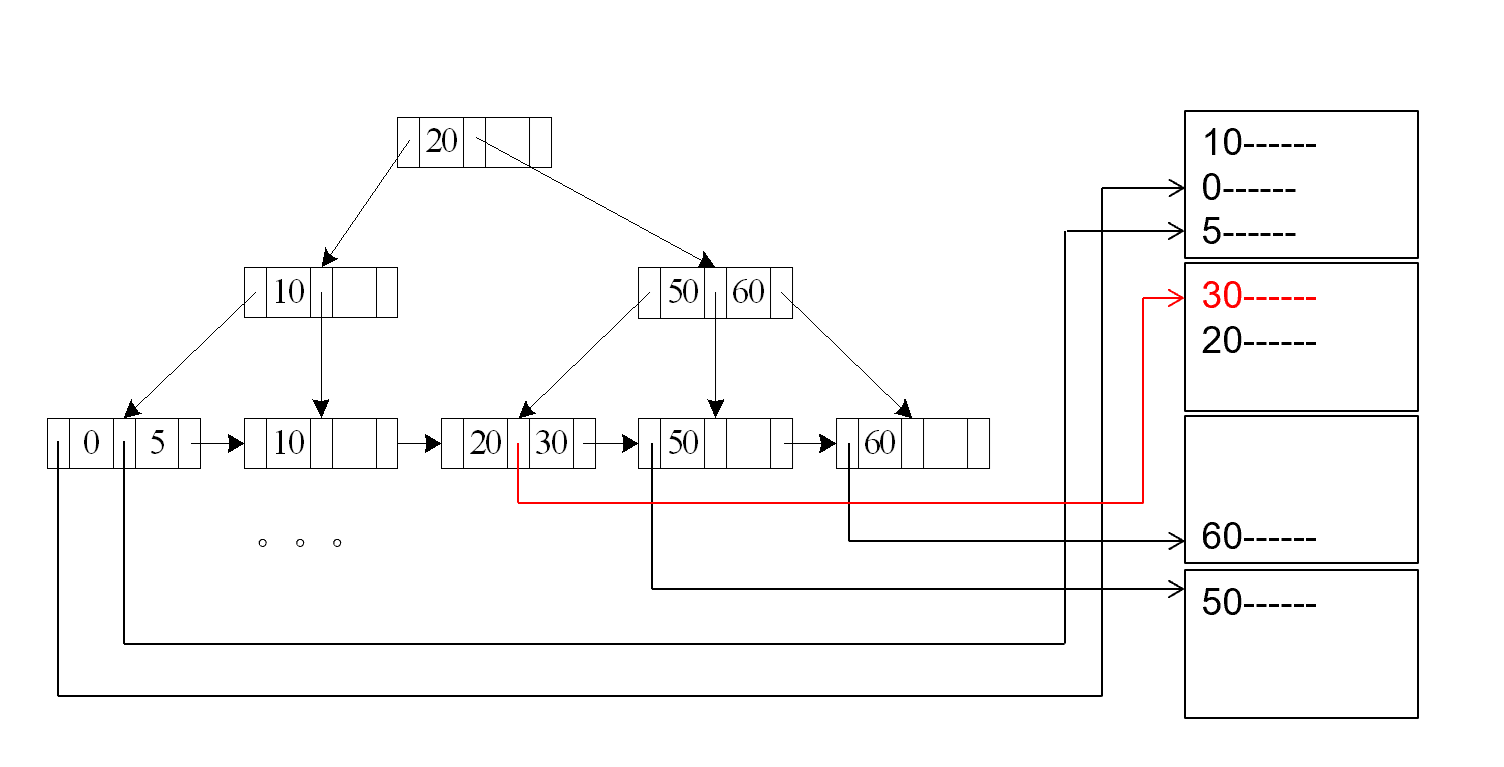
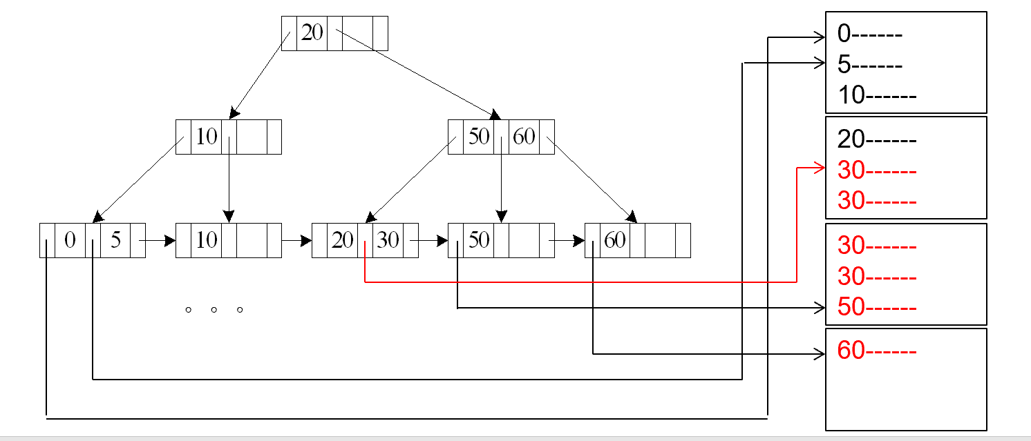
Sorting

For relations that don’t fit in memory, external sort-merge is a good choice.

Example

初始内存放不下，只能放 \(M\) pages. 一次性读 \(M\) 块，在内存内排序，排好后先写回，形成一个归并段。再读入第二段到内存中，排序后再写回，得到若干归并段(\(\dfrac{b_r}{M}\)) 会有 \(2*\dfrac{b_r}{M}\) 次 seek, \(2*b_r\) 次 transfer.

Procedure

Let \(M\) denote memory size (in pages).

• Create sorted runs(归并段)
  Repeatedly do the following till the end of the relation:
  • Read M blocks of relation into memory
  • Sort the in-memory blocks
  • Write sorted data to run \(R_i\); increment i. 假设生成了 \(N\) 个归并段

• Merge the runs

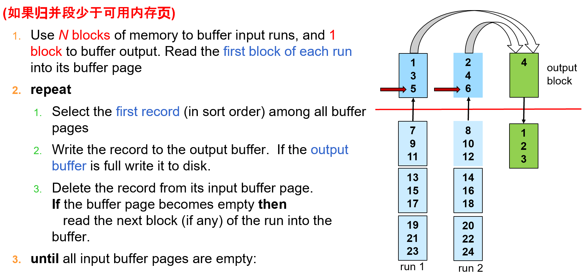
  • \(N<M\) 如果归并段少于可用内存页
    N 路归并
    归并时每一段只需要一块缓冲区（输出块也需要一块缓冲区）
    

    

  • \(N\geq M\)
    每次 pass, 我们不停地把 M-1 个段变成了一个大的归并段，此时数量减少为原来的 \(\dfrac{1}{M-1}\). 如果仍然数量超过 M, 继续 pass.
    e.g. If M=11, and there are 90 runs, one pass reduces the number of runs to 9, each 10 times the size of the initial runs.

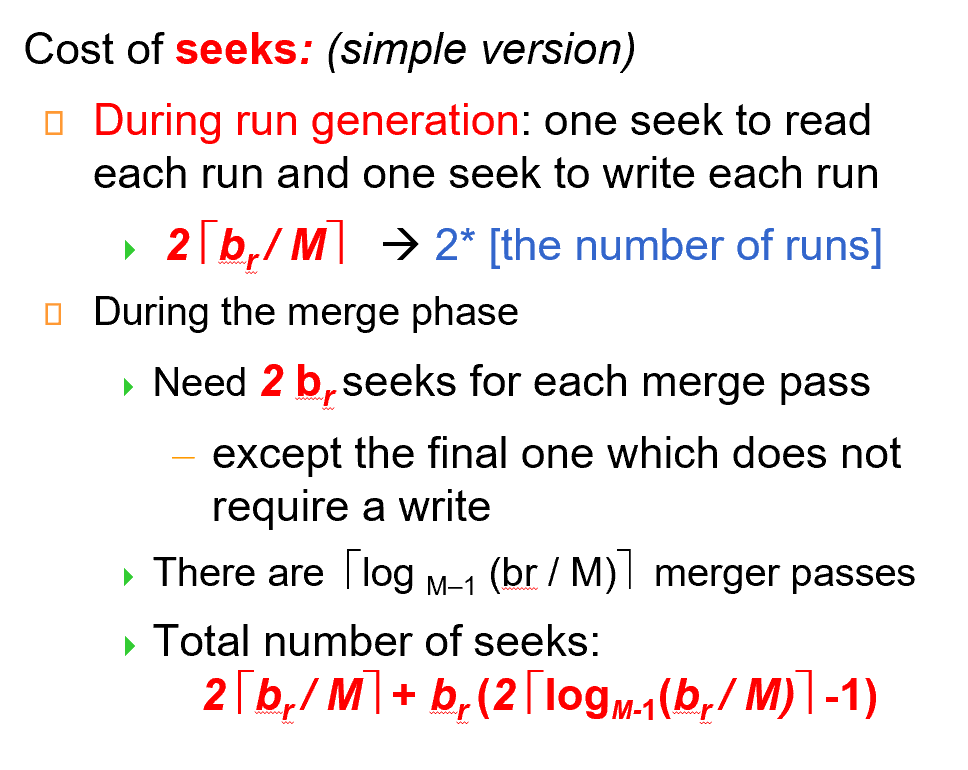
Cost analysis

• transfer

  

  我们不考虑最后一次写磁盘的 cost, 因为可能流水线会直接把结果交给下一步操作。 * seek

  

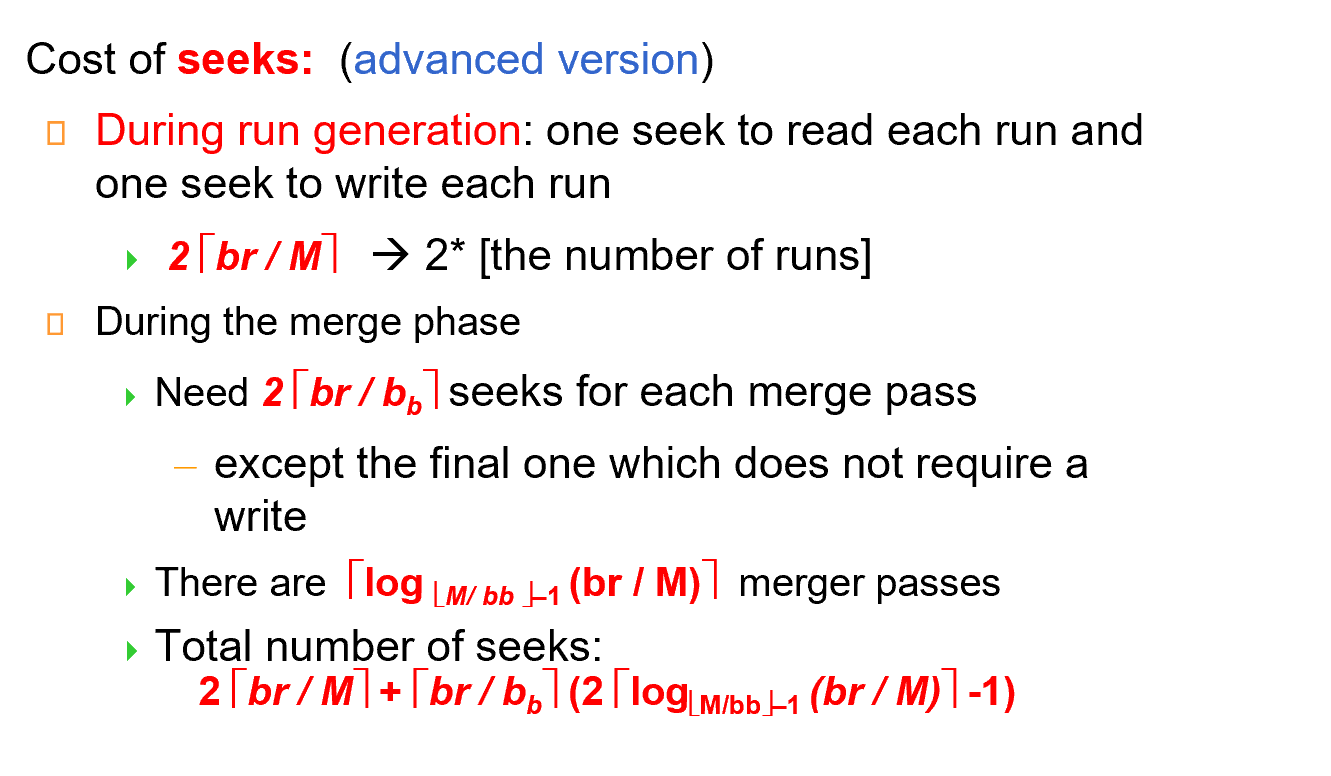
Advanced version

每一次读进去都要 seek, 可以改进。为每一个归并段分配多个缓冲区。这样我们定位一次之后可以读入多块进入缓冲区。
减少了 seek 次数，但这样轮次可能会增加。

Join Operation

Several different algorithms to implement joins

• Nested-loop join
• Block nested-loop join
• Indexed nested-loop join
• Merge-join
• Hash-join

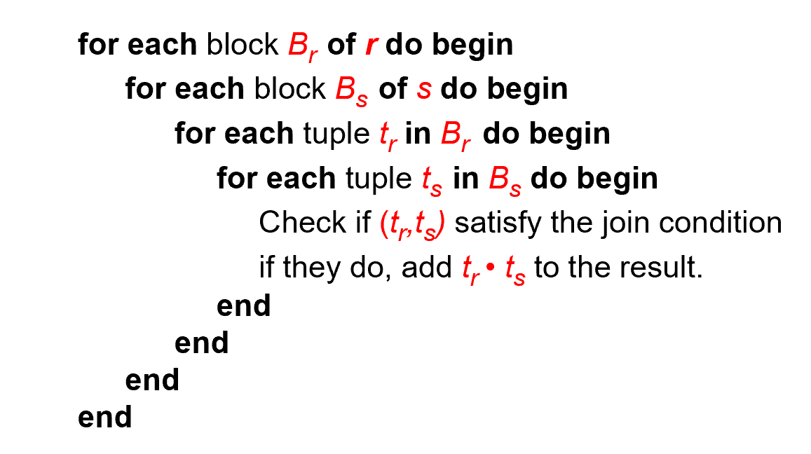
Nested-Loop Join

两重循环

• \(r\) is called the outer relation and \(s\) the inner relation of the join.

\(n_r * b_s + b_r\) block transfers, plus \(n_r + b_r\) seeks
对外循环每个记录，内循环的所有块都要进去. seek 时每次外循环都需要 seek, 内循环每轮只需要一次 seek.

如果内存能容纳所有的关系，那我们只需要 \(b_r + b_s\) block transfers and 2 seeks.

Block Nested-Loop Join

• Worst case estimate: \(b_r * b_s + b_r\) block transfers + \(2 * b_r\) seeks
  Each block in the inner relation \(s\) is read once for each block in the outer relation
• Best case: \(b_r + b_s\) block transfers + 2 seeks.

要把小的作为外关系。

Improvements to block nested loop algorithms:
假设内存有 M 块，有一块作为 output 的缓冲，剩下 M-1 块中 M-2 块均给外关系，内关系给一块。

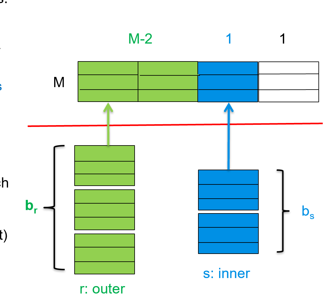
Cost = \(\lceil b_r / (M-2) \rceil * b_s + b_r\) block transfers + \(2 \lceil b_r / (M-2)\rceil\) seeks

• If equi-join attribute forms a key on the inner relation, stop inner loop on first match
  如果连接的属性是 key, 那么当我们匹配上之后就可以停止内循环。
• Scan inner loop forward and backward alternately, to make use of the blocks remaining in buffer (with LRU replacement)
  利用 LRU 策略的特点，inner 正向扫描后再反过来，这样最近的块很可能还在内存中，提高缓冲命中率。

Indexed Nested-Loop Join

如果内循环有索引，我们就没必要扫描内循环所有块了。

Index lookups can replace file scans if

• join is an equi-join or natural join and
• an index is available on the inner relation’s join attribute
  连接属性有索引

Cost of the join: \(b_r (t_T + t_S) + n_r * c\)
这里假定给外关系一块内存. \(c\) 表示遍历索引并取出所有匹配的元组的时间。

Merge Join

假设两个关系已经基于连接属性排好序，我们可以用归并的思想连接。

• Sort both relations on their join attribute (if not already sorted on the join attributes).
• Merge the sorted relations to join them
  • Join step is similar to the merge stage of the sort-merge algorithm.
  • Main difference is handling of duplicate values in join attribute — every pair with same value on join attribute must be matched

\(b_r + b_s\) block transfers + \(\lceil b_r / b_b\rceil + \lceil b_s / b_b\rceil\) seeks

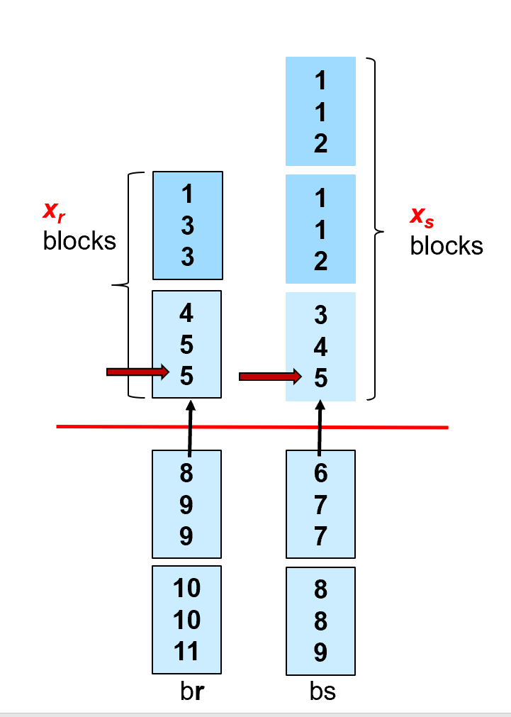
If the buffer memory size is M pages, in order to minimize the cost of merge join, how to assign M blocks to r and s respectively?

The estimated cost is \(b_r + b_s\) block transfers + \(\lceil b_r / x_r\rceil + \lceil b_s / x_s\rceil\) seeks (\(x_r+x_s=M\))

如果两个表都无序，我们可以先排序再 Merge-join, 这时还要算上排序的代价。

Hash Join

用一个 Hash 函数把两个关系进行分片。能够连接上的记录，一定处于同一个 partition 里面（反之不一定）
这样大关系变成了小关系。
我们要求其中某个的小关系要能一次放到内存中。

Applicable for equi-joins and natural joins.
the value \(n\)(partition 的个数) and the hash function \(h\) is chosen such that each si should fit in memory.
\(n \geq \lceil b_s / M\rceil\)
要求每个 partition 的大小都要小于 M, 不然不能一次性放进去。

如果我们的 \(n\) 很大，要分出来的 partition 很大，但是内存不够，关系分区不能一次生成所有的 partition, 要经过多次分区。
每次输入先被划分，随后进行细分。

注意分片的时候，还要写出去。
匹配时我们有哈希索引。

Typically n is chosen as \(\lceil b_s/M\rceil * f\) where \(f\) is a “fudge factor(修正因子)”, typically around 1.2
分不匀，我们有意放大。
The probe input relation partitions \(r_i\) need not fit in memory

Recursive partitioning

Recursive partitioning required if number of partitions n is greater than number of pages M of memory.

A relation does not need recursive partitioning if \(M > n_h + 1\), or equivalently \(M > (b_s/M) + 1\), which simplifies (approximately) to \(M > \sqrt{b_s}\).

Example

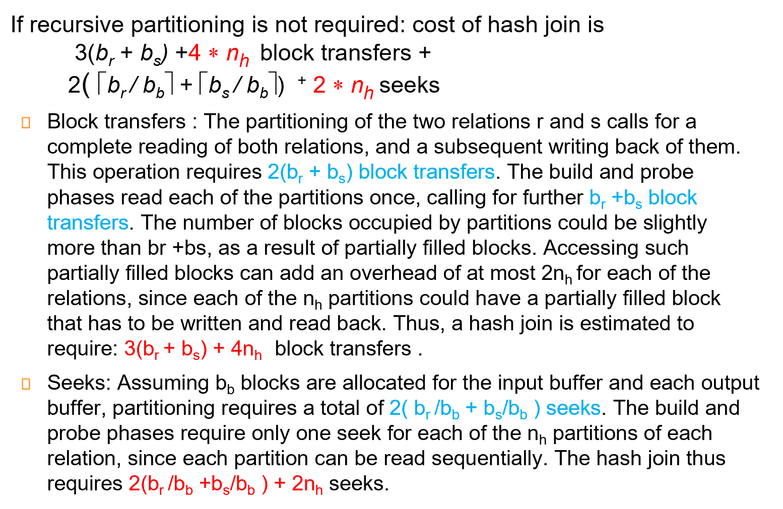
Cost of Hash-Join

Other Operations

• Duplicate elimination can be implemented via hashing or sorting.
  On sorting duplicates will come adjacent to each other, and all but one set of duplicates can be deleted.
  在排序的过程（生成、合并归并段就进行去重） Hashing is similar
• Aggregation
  Sorting or hashing can be used to bring tuples in the same group together, and then the aggregate functions can be applied on each group.
  生成归并段的时候，同一段的就可以统计统一结果

---

最后更新: 2023年5月25日 19:21:37
创建日期: 2023年5月25日 19:21:37

评论