Optimization

Introduction

• How do we find the best \(W\)?

  \[w^*=\arg\min_w L(w)\]

• 迭代改进

  • Random search (bad idea!)

    随机生成权重矩阵，计算损失，记录损失最小的矩阵。测试中只有 15.5% 的正确率。

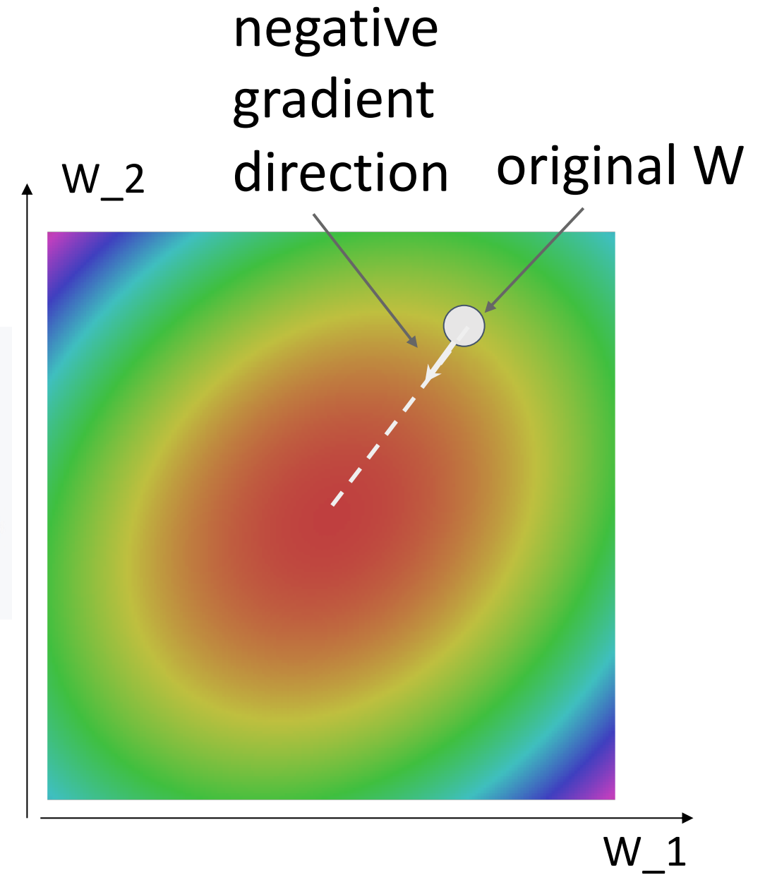
  • Follow the slope

    In multiple dimensions, the gradient is the vector of (partial derivatives) along each dimension.
    梯度就是函数增加值最快的方向。梯度的值告诉我们最大增加方向的斜率。

    所以我们朝负梯度的方向，向下降最大的方向移动。

• 如何计算梯度？

  • Numeric gradient: approximate, slow, easy to write.

    数字梯度，复杂度 \(O(\#dimensions)\).

  • Analytic gradient: exact, fast, error-prone.

    Loss is a function of \(W\). Use calculus to compute an analytic gradient.

  • In practice: Always use analytic gradient, but check implementation with numerical gradient. This is called a gradient check. e.g.torch.autograd.gradcheck gradgradcheck 分别用于检测一阶导和二阶导的正确性。

Gradient Descent

• Idea: Iteratively step in the direction of the negative gradient (direction of local steepest descent).

  w = initialize_weights()
  for t in range(num_iterations):
      dw = compute_gradient(L, data, w)
      w -= learning_rate * dw
  

  * Hyperparameters:
  • Weight initialization method
  • Number of steps

  • Learning rate

    我们对这个梯度有多信任，我们想要采取多大的步长。控制了网络学习的速度。较高的学习率表示你希望网络收敛更快。较低的学习率不太容易出现数值爆炸，但是需要更长的时间才能收敛。

Example

最开始的速度较快（因为梯度较大），当我们逼近底部的时候，收敛会变慢（接近平坦区域）。

• 我们讨论的梯度下降的版本实际上是 (Full) Batch Gradient Descent 批量梯度下降。

  \[ \begin{aligned} L & =\dfrac{1}{N}\sum\limits_iL_i(x_i, y_i, W)+\lambda R(W)\\ \nabla_W L(W)& = \dfrac{1}{N}\sum\limits_i\nabla_W L_i(x_i, y_i,W) + \lambda \nabla_W R(W) \end{aligned} \]

  批量是因为，损失是数据集里单个样本的损失的集合。因此可以看到梯度也是单个样本的梯度的集合。

  这可能会很昂贵，可能需要很长的时间来遍历整个数据集。实际中我们尝试用 SGD。

Stochastic Gradient Descent (SGD)

• Idea: 我们不再在整个训练数据集上计算总和，而是通过绘制完整训练数据集的小的子样本 (mini-batch) 近似梯度。

  每轮迭代只需要采样一小部分样本即可。

• Approximate sum using a minibatch of examples 32 / 64 / 128 common.

• Hyperparameters:

  • Weight initialization
  • Number of steps
  • Learning rate

  • Batch size

    Dont worry too much about the batch size, instead just try to make it as big as you can fit.

    批量大小，我们每个 mini-batch 有多少样本数量。常见的做法是让 mini-batch 尽可能大，直到用完 GPU 内存。

  • Data sampling

    not matter too much.

    常见的策略是在开始时对数据集进行打乱 (shuffle)，然后按顺序遍历数据集。

• 为什么叫随机：

  Think of loss as an expectation over the full data distribution pdata.
  我们的数据是从概率分布中采样而来的，相当于是进行了期望估计（蒙特卡洛估计）。

• Problems with SGD

  • What if loss changes quickly in one direction and slowly in another?
    在一个方向上变化非常快，在另一个方向上变化很慢。我们使用梯度下降，会发生什么？

    Example

    
    

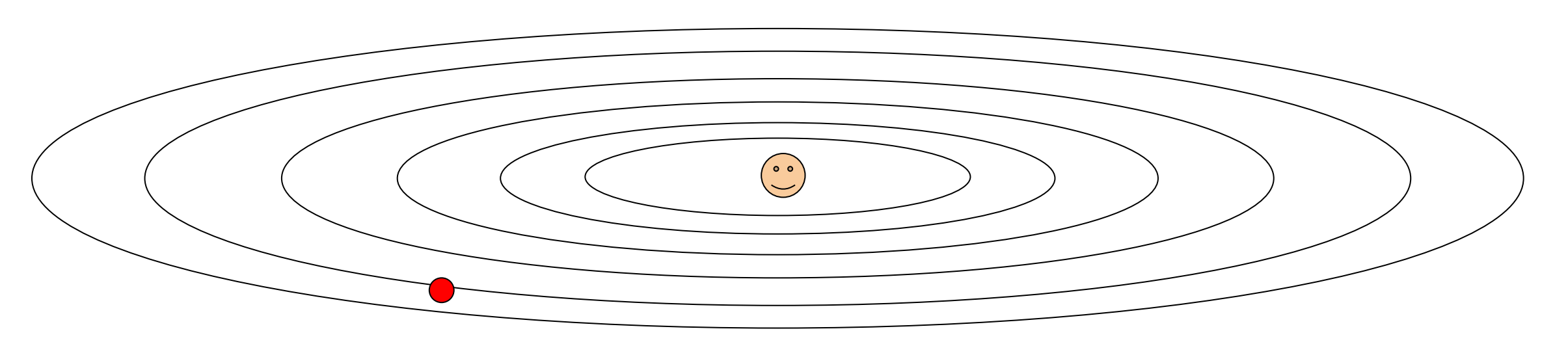
    Loss function has high condition number: ratio of largest to smallest singular value of the Hessian matrix is large.

    • 如果步长较大，会发生震荡，会需要更多的步数。
    • 我们如果把步长设得很小，可以避免震荡，但会导致收敛非常慢。

  • What if the loss function has a local minimum or saddle point?

    • 局部最小（梯度为 0，但却不是函数的最低点），这种情况我们可能会在局部最小点停下，因为这里的梯度为 0，所以我们的步长也为 0.
    • 鞍点：在一个方向上函数增加，另一个方向上降低。这个鞍点的梯度也为 0. （高维优化中易出现）
    Exapmple

    
    

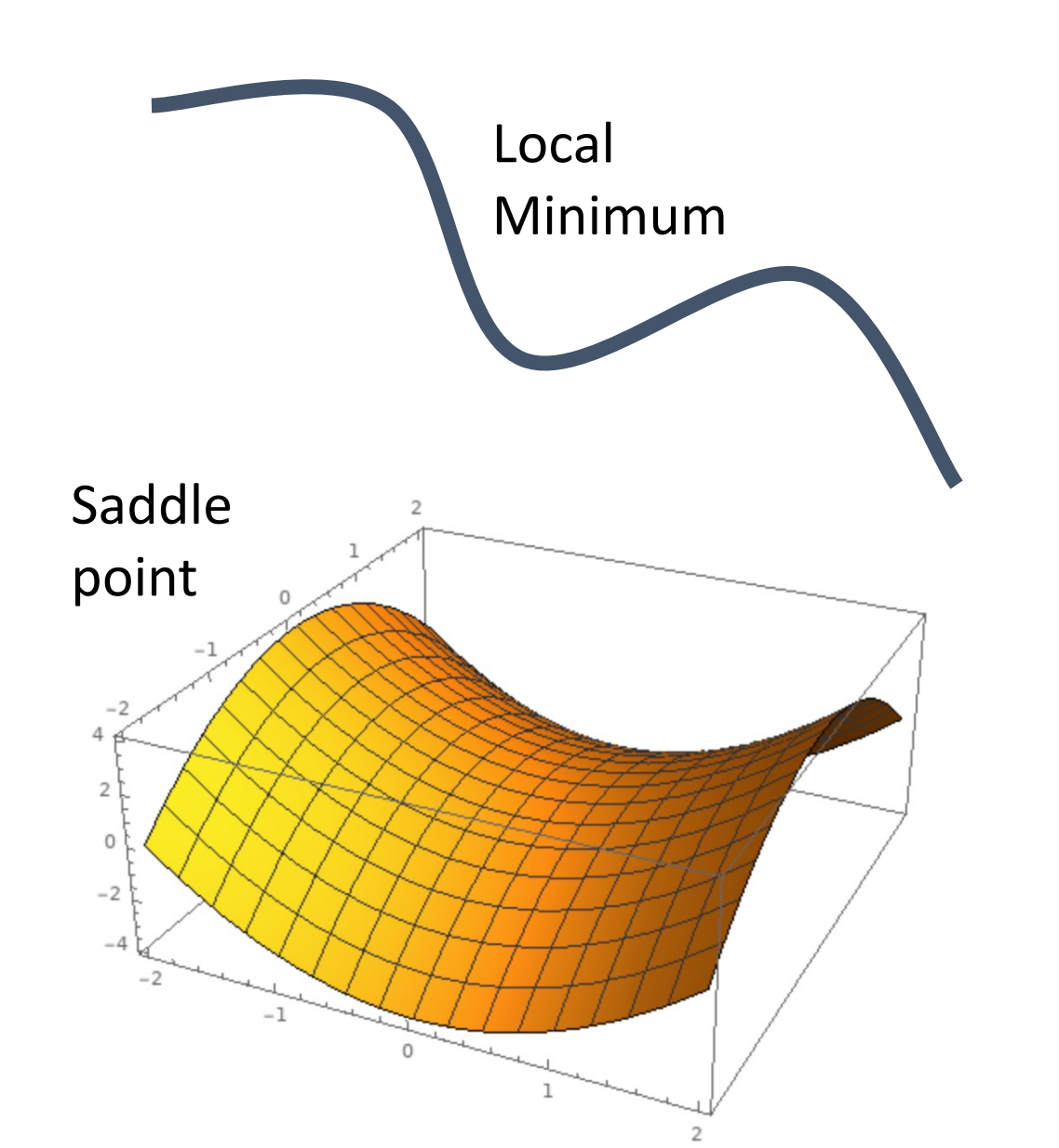
    Zero gradient, gradient descent gets stuck.

  • stochastic part

    Our gradients come from minibatches so they can be noisy!

    噪声可能导致用于更新的梯度可能与我们想要到达的真实方向没有很好的相关性。

SGD+Momentum

• Idea:

  • Build up “velocity” as a running mean of gradients
  • Rho gives “friction”; typically rho=0.9 or 0.99

  想象一个球加速下坡的时候，他会获得加速度。尽管局部梯度没有直接与它的运动方向对齐，它也会继续沿着该方向移动。 * 算法有不同版本，但下面的公式实际上是等价的。

  

  You may see SGD+Momentum formulated different ways, but they are equivalent - give same sequence of x.

• 如何解决 SGD 的三个问题：

  • 尽管到达了局部最小，但是依然有速度，可以继续移动。鞍点
  • 速度相当于加权平均了我们在训练期间的所有梯度。如果出现了震荡的情况，速度矢量有助于平滑这一点。
  • 可以平滑噪声。

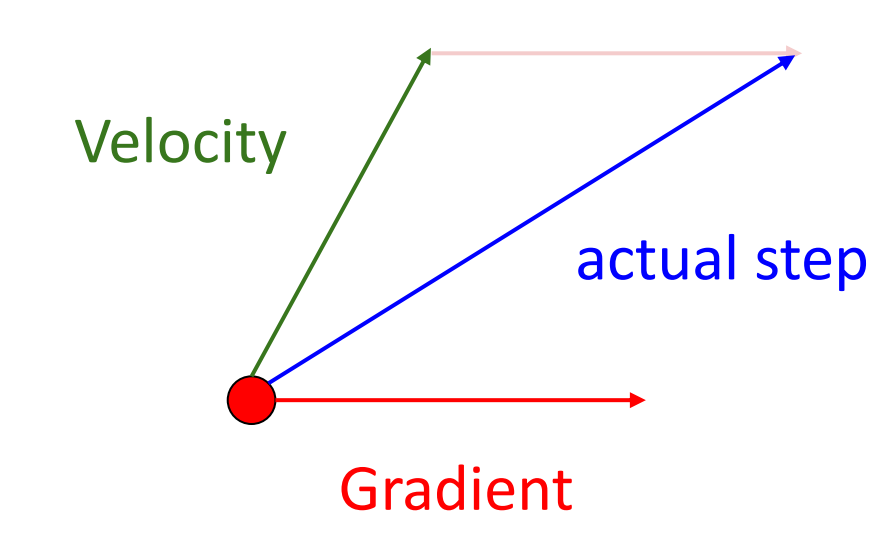
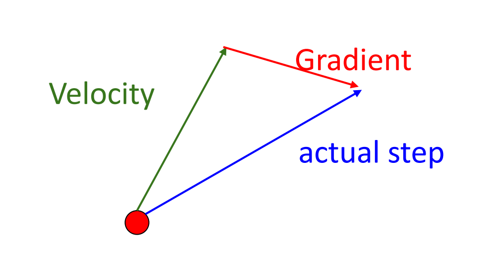
• 思考动量更新：Combine gradient at current point with velocity to get step used to update weights.

  
  

  Nesterov Momentum 另一种形式:

  
  

  “Look ahead” to the point where updating using velocity would take us; compute gradient there and mix it with velocity to get actual update direction.

  从当前点向前看（根据当前速度），随后在那里计算梯度并和速度混合得到真正的更新方向。

  \[v_{t+1}=\rho v_t - \alpha \nabla f(x_t+\rho v_t), x_{t+1}=x_t+v_{t+1}\]

  Annoying, usually we want update in terms of \(x_t, \nabla f(x_t)\)

  我们一般是根据当前点进行优化，使用一个变量替换 \(\widetilde{x_t}=x_t+\rho v_t\) 就可以改写为当前位置的形式。

AdaGrad

我们依然希望找到一些其他办法来克服 SGD 的问题。

• Idea: Added element-wise scaling of the gradient based on the historical sum of squares in each dimension.

  这里我们不再跟踪梯度的历史平均值，而是追踪梯度平方的历史总和。当我们迈出下一步时，我们会除以这个历史总和的平方根。

  • Progress along “steep” directions is damped; progress along “flat” directions is accelerated

  当梯度变化非常快时，我们会除以一个大值，有助于抑制梯度变化的速度；当梯度变化非常慢时，我们会除以一个小值，相当于在当前方向加速运动。

  • 长时间运行 AdaGrad 会发生什么：梯度平方会不断累积，并可能停止继续运动。

• Code:

  grad_squared = 0
  for t in range(num_iterations):
      dw = compute_gradient(L, data, w)
      grad_squared += dw**2
      w -= learning_rate * dw / np.sqrt(grad_squared + 1e-7)
  

RMSProp: “Leaky Adagrad”

• Idea: 有摩擦系数，会使得梯度平方和不断缩减。
• Code:

  grad_squared = 0
  for t in range(num_iterations):
      dw = compute_gradient(L, data, w)
      grad_squared = decay_rate * grad_squared + (1 - decay_rate) * dw**2
      w -= learning_rate * dw / np.sqrt(grad_squared + 1e-7)
  

Adam (almost): RMSProp + Momentum

• What happends at t=0? (Assume beta2=0.999)

  会得到接近 0 的平方根（在分母下面）

  
  

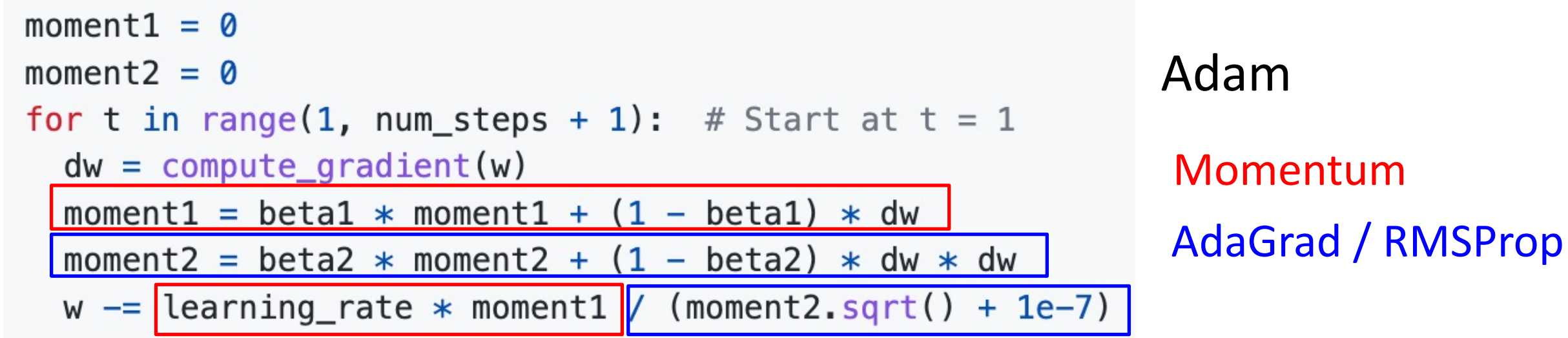
• Idea: 优化的开始我们希望建立对第一和第二动量的稳健估计。

  
  

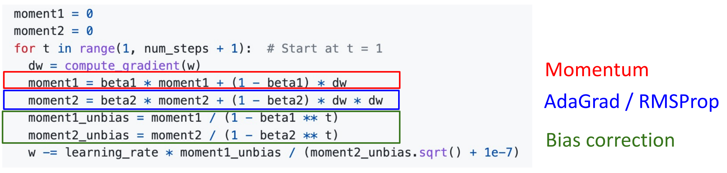
  Bias correction for the fact that first and second moment estimates start at zero.

• Adam with beta1 = 0.9, beta2 = 0.999, and learning_rate = 1e-3, 5e-4, 1e-4 is a great starting point for many models!

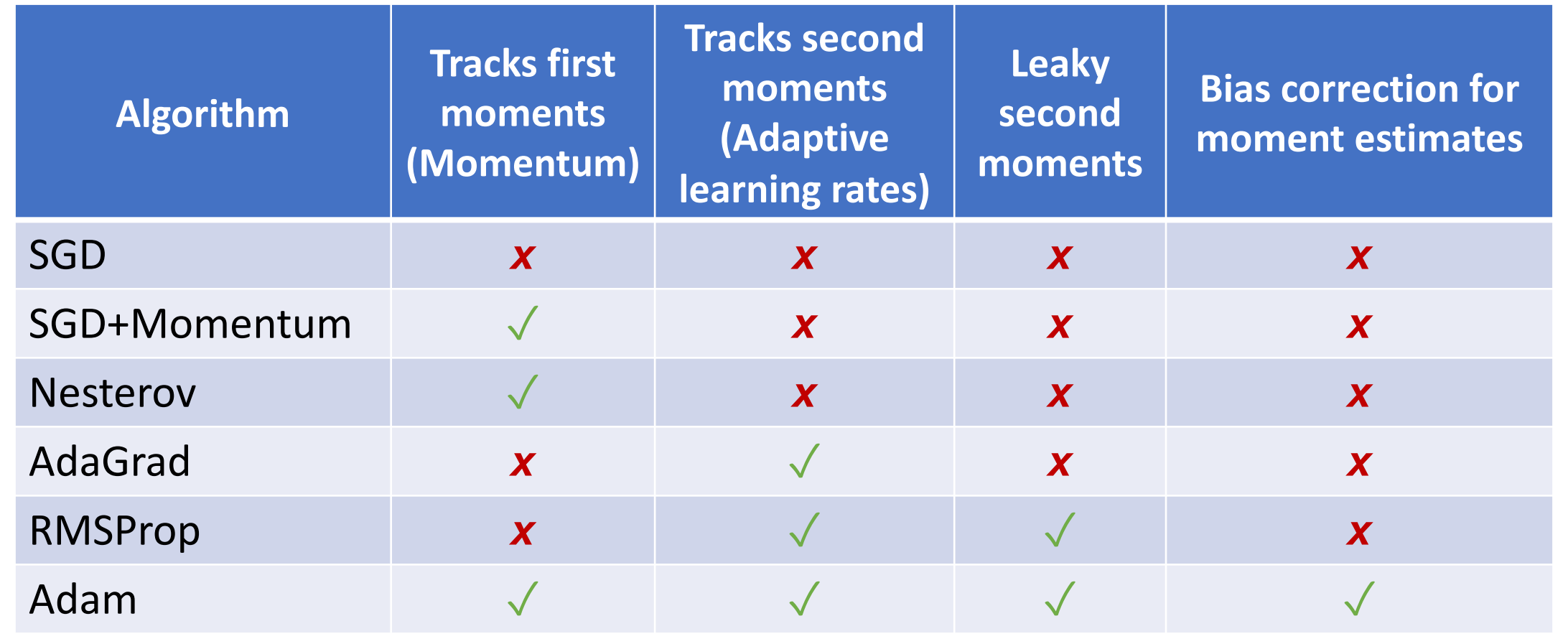
Adam: Very Common in Practice!

Optimizers

Second-Order Optimization

• So far: First-Order Optimization.

  到目前为止只用了梯度（一阶导数）信息，步骤如下：

  1. Use gradient to make linear approximation
  2. Step to minimize the approximation

• Use gradient and Hessian to make quadratic approximation.

  可以使用二阶导数来做优化，让算法自适应地选择要走多长的步子。（根据曲率选择）

  \[ \begin{aligned} L(w) & \approx L(w_0)+(w-w_0)^\top\nabla_w L(w_0)+\dfrac{1}{2}(w-w_0)^\top H_w L(w_0)(w-w_0)\\ w^* & = w_0 - H_wL(w_))^{-1}\nabla_w L(w_0) \end{aligned} \]

• Why is this impractical?

  Hessian has \(O(N^2)\) elements Inverting takes \(O(N^3)\) \(N=\) (Tens or Hundreds of) Millions.

  高维空间下 Hession 矩阵会很大。我们要求 H 的逆，需要更大的空间。

  低维空间可以使用，高维空间 impractical.

• In practice:

  • Adam is a good default choice in many cases SGD+Momentum can outperform Adam but may require more tuning.
  • If you can afford to do full batch updates then try out L-BFGS (and don’t forget to disable all sources of noise).

Summary

Summary

• Use Linear Models for image classification problems
• Use Loss Functions to express preferences over different choices of weights
• Use Regularization to prevent overfitting to training data
• Use Stochastic Gradient Descent to minimize our loss functions and train the model

---

最后更新: 2024年3月23日 19:26:25
创建日期: 2024年3月23日 19:26:25

评论